Organization
1. Packet Switched (PS) Network
2. Netwrok Perfomance Analysis
3. PS Switched Network
4. Types of Delay
5. Packet Loss
6. Throughput
7. Stop & Wait / window / small and large window protocol
8. Goodput
In order to use the resources in a network efficiently, we send the information in packets. Network resources are the bandwidth and the switching elements such as routers. In packet switching all users use these resources jointly.
Packet Switched (PS) Network
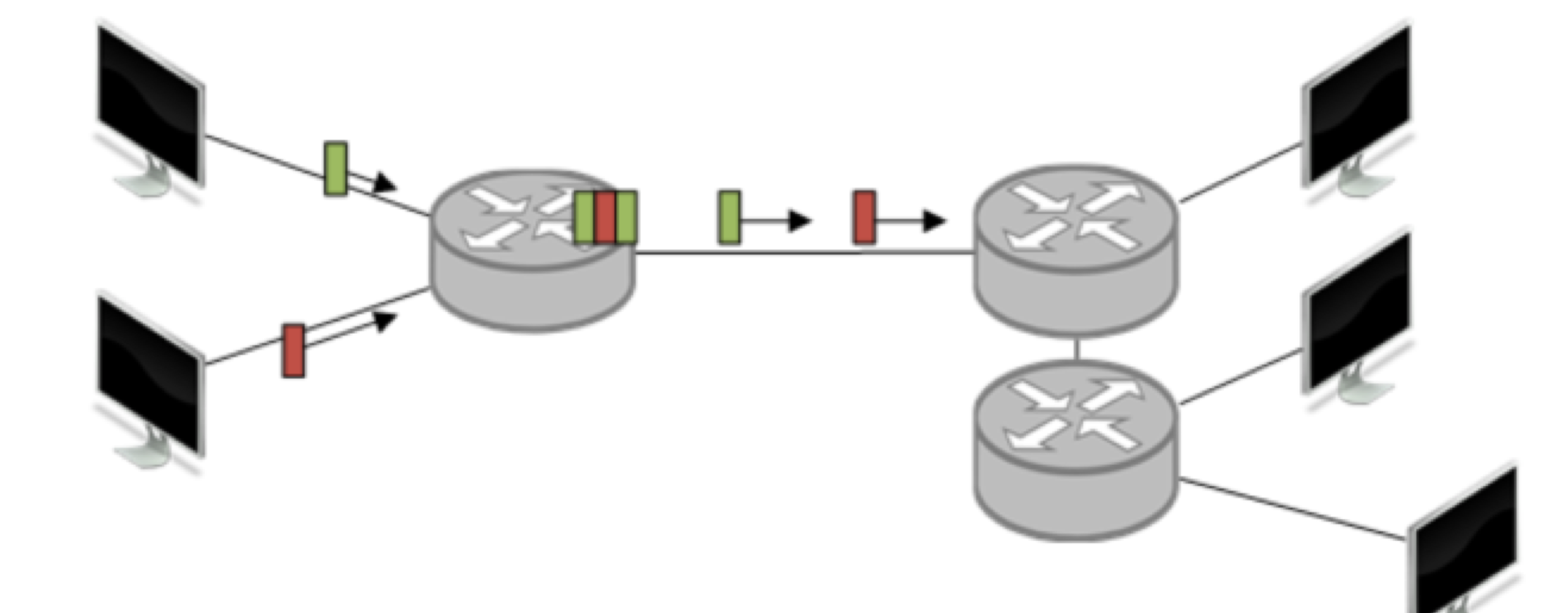
For Packet Switching the information packets have to be forwarded in each network node towards their destination.
- A typical network node : joint usage of resources such as a router or a bandwidth.
- Multiplexing gain.
- Underlying Principle : Stroe and Forward. - Packets are queued in the buffer of a network node before processing and forwarding.
- This principle affects performance of network.
- packets are buffered (= delay)
- buffer overflow (= loss)
Netwrok Perfomance Analysis
We can observe this behavior every day with applications in the Internet, when we are exposed to waiting times.
Performance Metrics of Packet Switched Networks
- Delay : the latency that a packet obtains from traversing a network
- Packet Loss : the fraction of packets that is lost while traversing the network
- Throughput : the amount of traffic that can traverse the network per time unit
Types of Delay
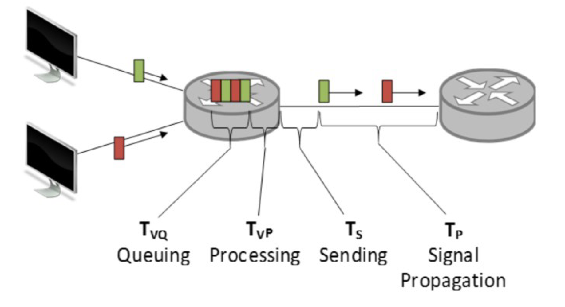
- An ncoming packet to a router is queued in the buffer.
- The packet is taken from the buffer after some waiting and processed (destination address is checked, the routing path is determined.)
- The packet is sent out on the network. The sending time lasts from the first bit of the packet until the last bit.
- The corresponding signal on the medium then takes a propagation time until it reaches the next network node.
| 1. Queuing | 2. Processing |
| $$ T_{VQ} $$ | $$ T_{VP} $$ |
| - Wait in butter until packet can be processed - Depends on the load of the system -it can be significant |
- Check on errors - Routing decision - Usually some \(\mu s \) |
| 3. Sending | 4. Signal Propagation |
| $$ T_{S} = \cfrac{\mathbf{L}}{\mathbf{R}}$$ | $$ T_P = \cfrac{d}{c} $$ |
| - Time to send packet on media - Depends on Data/rate \(\mathbf{R}\) and packetlength \(\mathbf{L}\) - Significant for small \(\mathbf{R}\) |
- Propagation time on the media - Depneds on speed of light in the media \(c\) and distance \(d\) - Few \(\mu s\) up to 100 ms |
Here is a the four delay types in a message sequence chart.
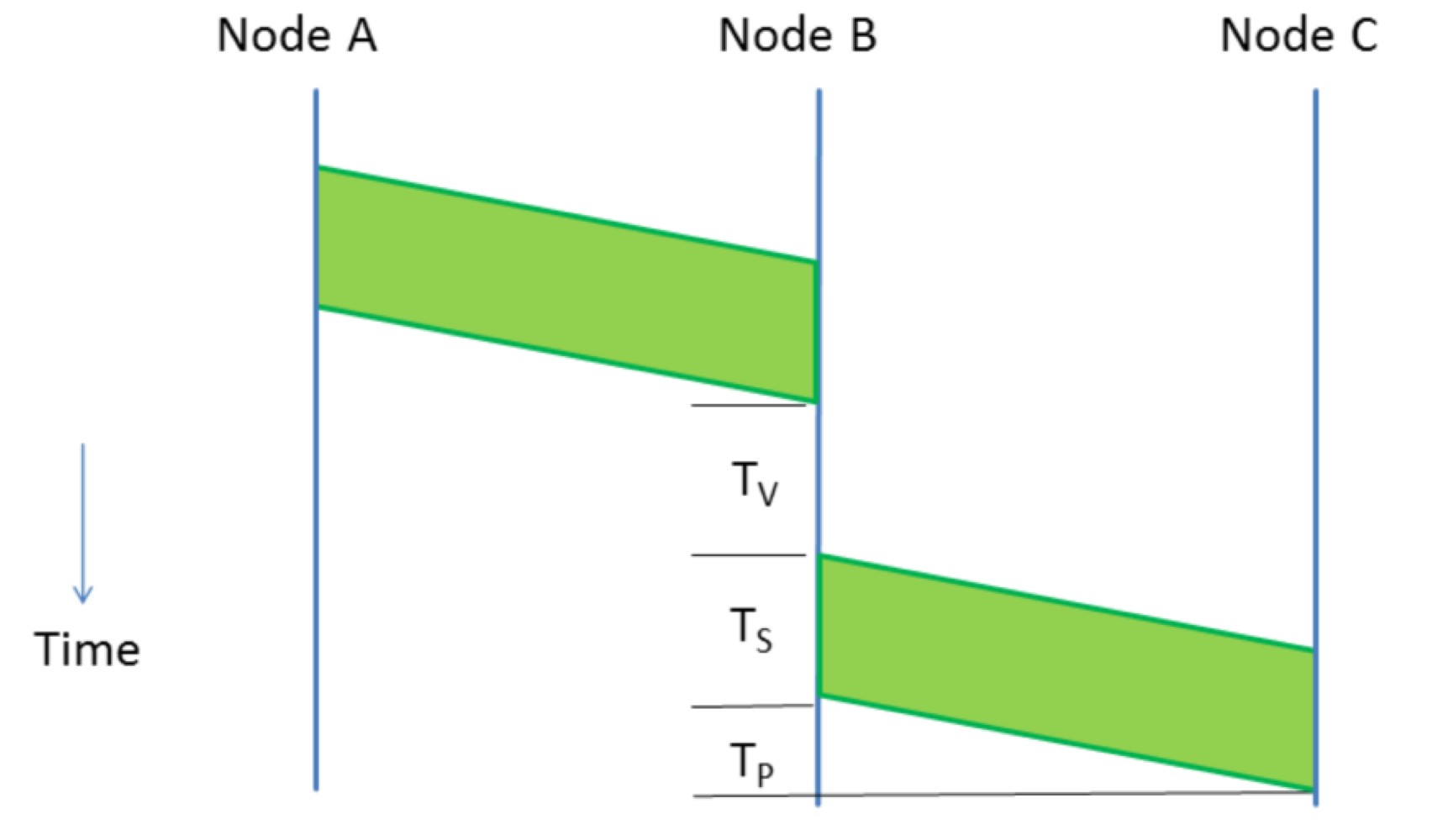
The total delay from the arrival of the last bit at the middle node B to the arrival of the last bit of the packet on the next node C is t the sum of all delay types.
$$\mbox{Total delay : } T_{total} = T_{Vqueue} + T_{Vproc} + T_S + T_P $$
$$ \qquad T_V = T_{Vqueue} + T_{Vproc}$$
Delays and where they come from
| Sending Time \( T_S\) | Pretty constant : Only depends on packet length, computing power etc |
| Propagation Time \( T_P\) | |
| Processing Time \( T_{VP}\) | |
| Queuing delay \(T_{VQ}\) | Highly load dependend : depends on the arrival rate of the packets and the distribution of the arrival process |
Packet Loss and Queuing Strategies
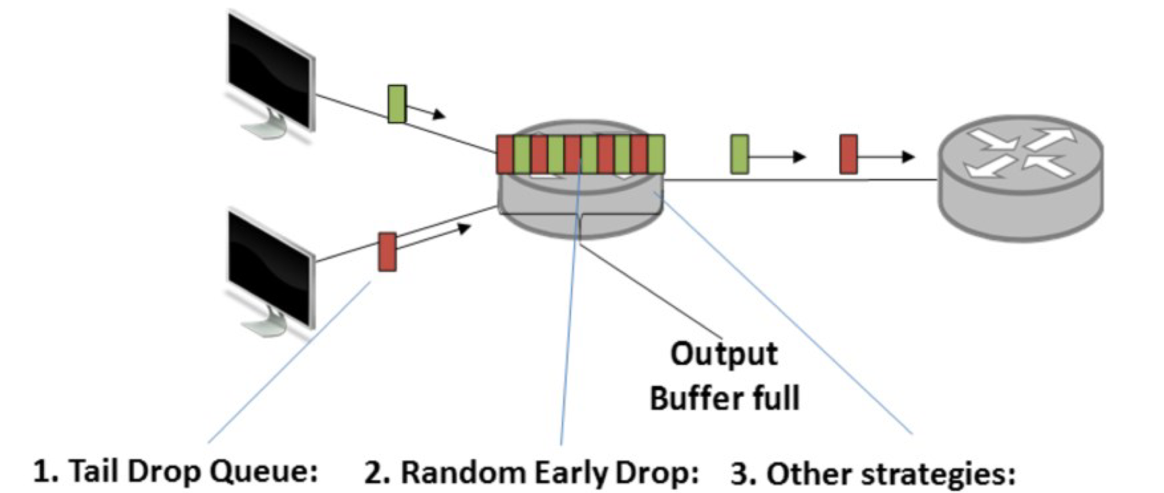
- Packet loss depends on the incoming traffic rate and on the buffer size, and the buffer is limited.
- If the buffer is full \(\rightarrow\) packets are dropped from the queue and are lost.
- Lost pakets can be retransmitted by the preceding node or by the sender or not at all.
Queing Strategies:
1. Tail Drop Queue : Drop arriving Pakets
2. Random Early Drop : Drop randomly chosen packets from the buffer
3. Other strategies : Priority Queue, Weighted Fail Queue etc.
Throughput and Efficiency

The Throughput (TP) describes the speed of data transmission between sender and receiver that is achievable over a longer time interval.
Rate is the transmission speed "on the wire"
TP considers efficiency of the protocol
| Throughput | Utilization |
| $$TP = R * \rho $$ | $$ \rho = \cfrac{\mbox{sending time of successfully transmitted packets}}{\mbox{total duration of the transmission process}}$$ |
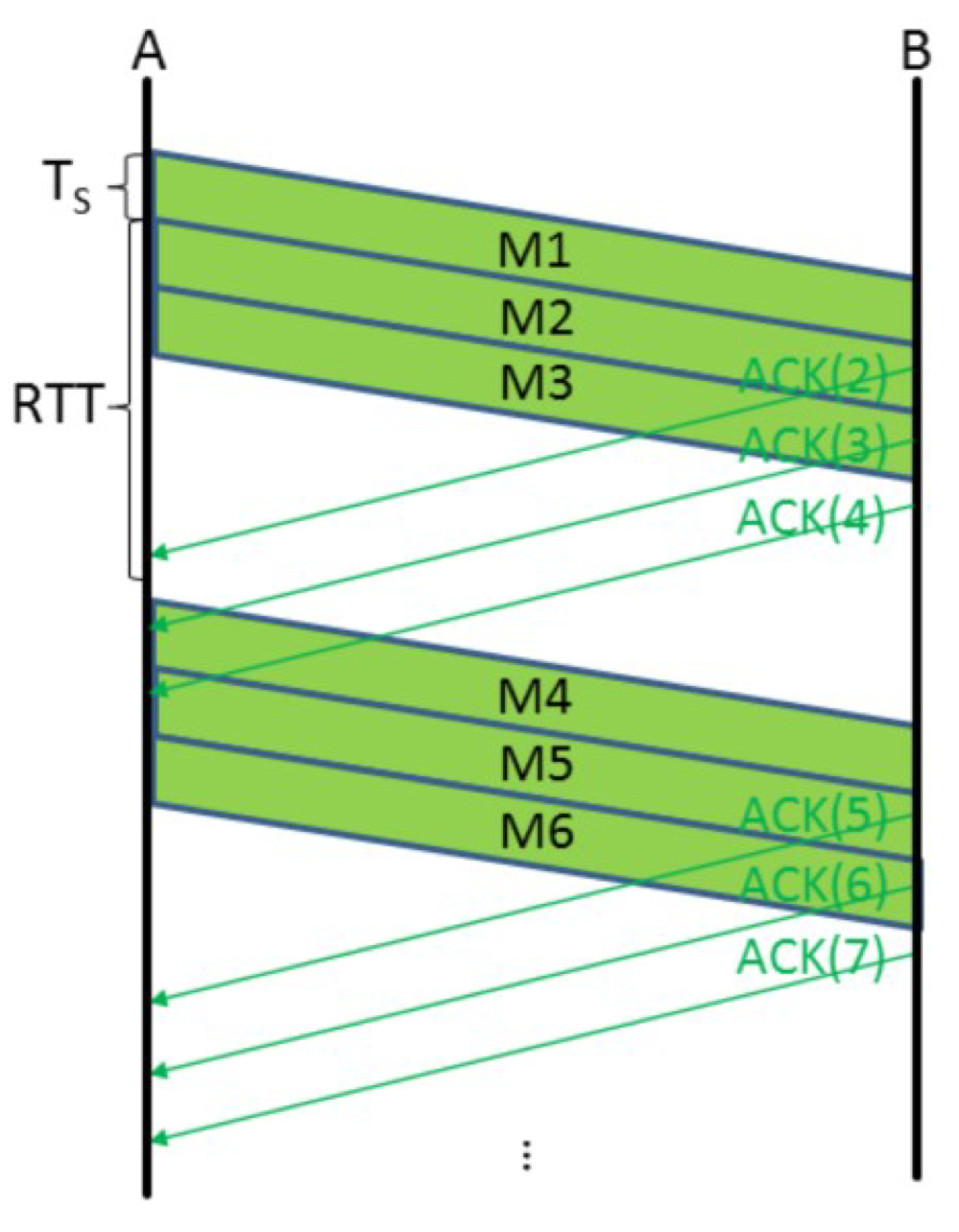
Stop & Wait Protocol
The Stop and Wailt protocol follows a simple principle to achieve successful transmissions.
To make sure that packets have arrived at the destination,
(1) the sender waits for an acknowledgement by the receiver.
(2) Only if an Acknowledgement is received the next packet is sent.
In this way the stop and wait protocol does not fully utilize the link data rate.
The utilization
$$ \rho_{\mbox{stop&wait}} = \cfrac{\mbox{packet sending time}}{\mbox{total time for transmission (with ACK)}} $$

In this example the utilization is the sending time of one packet divided by the total time for transmission that is the sending time \(T_S\) + the round trip time RTT. The round trip time is twice the propagation delay \(T_P\) once from A to B and once from B to A and twice the processing time \(T_{VP}\) , one time at each node.
$$ \mbox{The utilization : } \rho_{\mbox{stop&wait}} = \cfrac{T_S}{T_S + RTT} = \cfrac{T_S}{T_S + 2 \cdot T_V + 2 \cdot T_P}$$
Window Protocol
In order to increase the utilization, more packets have to be sent before an acknowledgement is received.
 |
Sender allow more than one message to be in flight, up to \(w_{s, max} messages can be not acknowledged at a time\) \(\bullet \) Here: \(w_{s, max} = 3 \) \(\bullet \) Messages are sent in groups \(\bullet \) Utilization can be increased $$ \rho_{\mbox{window}} = \cfrac{w_{s, max} \cdot T_S}{T_S + RTT} $$ |
Small and Large Windows
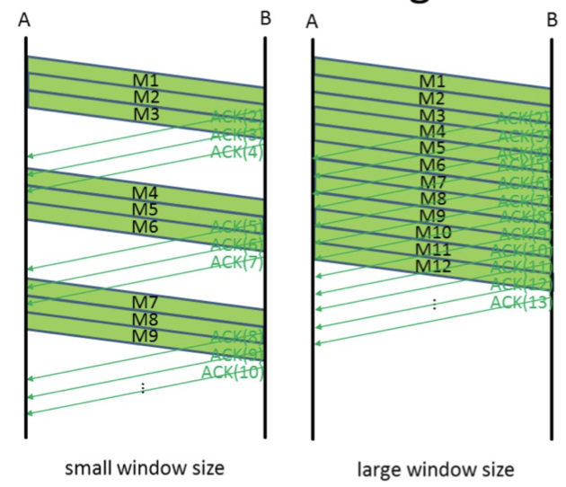
When we consider this window protocol principle further then we can see what with a large enough \(w_{s, max} \) we can achieve an utilization of 100%.
$$\rho_{window} = \cfrac{w_{s, max} \cdot T_S}{T_S + RTT}$$
$$ \quad \rightarrow W = \left\vert \cfrac{T_S + RTT}{T_S} \right\vert $$
An important measure to determine the optimum window size is the Bandwidth Delay Product. The window size is depending on the sending time and the round trip time.
If we write the details for the round trip time, replace \(T_S\) by \(L\) over \(R\) and multiply enumerator and denominator with the data rate then we see that the optimal window size depends on the product of \(R\) and the propagation delay. This is the Bandwidth Delay Product.
$$ W \sim \cfrac{T_S +RTT}{T_S} = \cfrac{T_S + 2 \cdot T_V + 2 \cdot T_P}{T_S}
$$ = \cfrac{\cfrac{L}{R} + 2 \cdot T_V + 2 \cdot T_P}{\cfrac{L}{R}} $$ = \cfrac{L + 2 \cdot T_V \cdot R + 2 \cdot R \cdot T_P}{L} $$
$$ \rightarrow W \sim R \cdot T_P $$
$$ \mbox{Networks with a large Bandwidth Delay Product need a large sendling window}$$
Even if \( \rho = 100%\)? We call this "Goodput"
Goodput
\(\rightarrow\) a high throuput \(\rightarrow\) header overhead in each packet
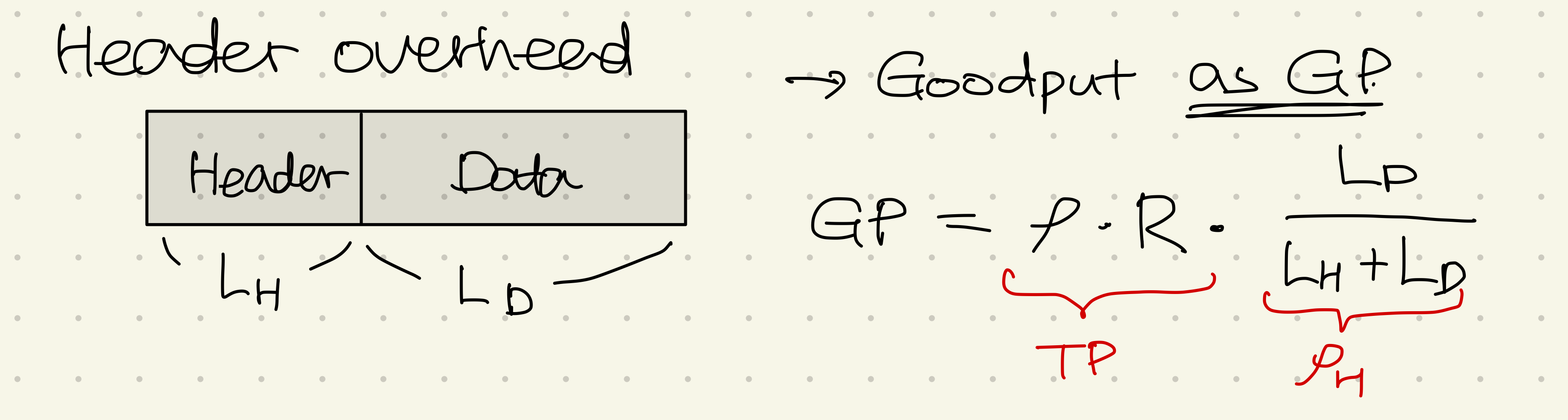
Each packet consists typically of a header of length LH and the user data of length LD. The header contains addresses, sequence numbers and other control related information.
We have to substract the header from the user data to get the real effective throughput.
We call this the Goodput.
The Goodput is the Throughput multiplied by the fraction of the user data length over the total packet length.
Please note that in the case of packet loss for the effective throughput also the retransmissions have to be considered and lead to a lower utilization and hence a lower throughput or goodput respectively.

'All About ECE > Communication Networks' 카테고리의 다른 글
| [Data Networking] MAC and PHY layers (0) | 2023.01.16 |
|---|---|
| [Data Networking] Traffic Theory - a brief introduction (0) | 2023.01.15 |
| [Data Networking] Protocols, OSI Protocol Stack (0) | 2023.01.13 |
| [Commu-Network/정보통신망] Message Transfer : Nachrichtenaustasuch (1/2) (0) | 2022.12.25 |
| [Commu-Network/정보통신망] Information Transfer : Informationsübertragung (2) | 2022.12.24 |


댓글