Organization
1. Traffic Theory for Queuing Systems
2. Model of an Internet Router & Random Process
3. Offered Traffic
4. Stability Condition
5. Markow Chains of Queuing Sysems States
6. M/M/1 Queuing System
7. M/M/N Queuing System
9. M/M/N/0 Loss System
Traffic theory allows us to calculate performance metrics for communication networks from analytical models.
- Queuing Models: analytical models to calculate performance metrics of communication networks
- Focus : single packet forwarding node (router, switch)
- Performance metrics :
(1) Probability of x packets in service
(2) Average number of packets in service
(3) Average queue length - buffer fullness
(4) Average queuing delay
(5) Packet loss probability
Model of an Internet Router
Let's think about Internet Router. What is the process of Internet Router?
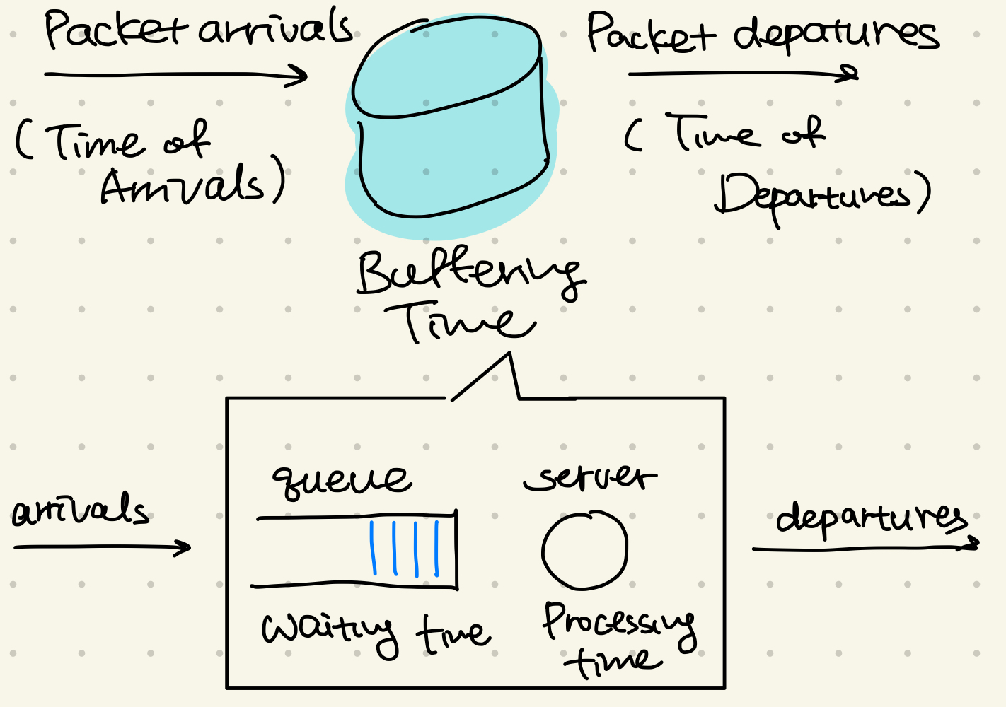
A simple model might look like this. The router consists of a buffer, which casus watigin time ofr those packets are queued. We can detail this simple model.

The arrivals are characterized by an arrival process with a meann arrival rate Lamda. Such an arrival process might be modeled by a Poisson process for example. We denote the buffer by its size s of maximum packets it can buffer and the server part of a router by its N service units with a service process and a service rate \( \mu\)
- Arrivals and servings are in general without rules i.e. RANDOM!
- arrival process / service process : The time sequence of such arrivals and servings is calles arrival process respectivelyy service process.
- state process : Arrivals and servings change the system state - e.g. the number of occupied servers or filled buffer units.
- state process \(X(t)\) : number of occupied units - serving & buffer units.
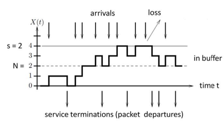
Such state process is illustrated on the upper right side. Our model is: N = 2, s = 2.
- With each arrival = arrows coming from above the value of X increases by one.
- With each service termination, that is a packet departure, the value of X is decreased by one.
- If there are arrivals when all serving units and all buffer units are occupied, that is when X has the value of 4, arriving packets are lost as they cannot be served or buffered by the router.
Offered Traffic
The offered traffic corresponds to the man traffic load in the system if no loss occurs.
$$ A = \cfrac{\lambda}{\mu} = \lambda h $$

It is defined by the relation of the mean arrival rate and the mean departure rate with respect to one server unit.
And we measure it pseudo unit "Erlang (Erl)" , without dimension
- 1 server continously in use : 1 Erl
- for > 1 server units offered traffic can be > 1 Erl
- if offered traffic is > 1 Erl for one server unit \(\rightarrow\) loss
$$ \mbox{Utillization : } \rho = \cfrac{A}{N} \qquad A = N_P \qquad N \mbox{ : number of server units}$$
So 1 Erlang means that one server continously occupied.
Stability Condition
Also we can easily conclude that the offered traffic has to be below the system performance capabilities. That means the offered traffic has to be lower than the number of server units N. We call this the stability condition for a queuing model.
$$ \mbox{Stability condition } A < N $$
$$ \mbox{For the utilization} \qquad \rho = \cfrac{A}{N} \quad \rho < 1 $$
Here is an example. Let us assume a router with 1 Mbit/s ougoing link. This characterizes the departure rate. Further we have 35 users and each of them generates traffic of a mean data rate of 100 kbits/s and each user only active 10% of the time. Then
the offered traffic : \( A = 35 \cdot 0,1 \cdot 100\)kbits/s , and divide with 1 Mbit/s
Then A = 0,35 and it is smaller than 1 , and it means stability condition OK.
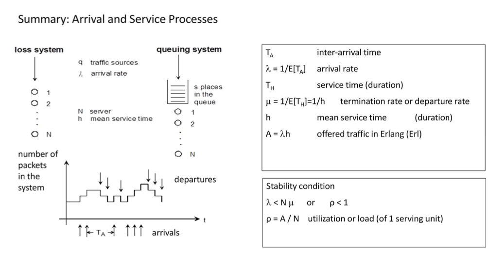
Let me summarize what we have learned so far: We model a network forwarding node such as an Internet router. In the model it consists of a buffer, where arriving packets are queued until they are processed, and server units. The buffer has a size of s buffer units. There are N server units or servers. Each server is characterised by a mean service time h which is the same as 1 over the departure rate \(\mu\). The traffic is emerging from q traffic sources and is characterizes by a total average arrival rate \(\lambda\). The service X describes the number of packets in the system at a given time t depending on arrival and departure events.
In case we do not have a buffer, arriving packets are lost if all N server units are occupied. We call this a loss system. In case the number of buffer units s is larger than zero, we call our model a queueing system.
On the right side, we summarize the main elements of our model. \(\lambda\) is the mean arrival rate, given by 1 over the expected value ot the inter‐arrival time. \(\mu\) is the mean departure rate given by 1 over the expected value of the time a packet is in service by a server. Instead of \(\mu\) we sometimes use h for the mean service time.
A is the offered traffic. It is the product of the mean arrival rate and the mean service time or the division of the mean arrival rate and the mean departure rate.
Our system model is stable if the mean arrival rate is smaller than N times the departure rate. The utilization is the offered traffic per service unit and is defined as the division of the offered traffic A by N
Kendall Notation for Queuing Models

we use Kendall Notation in order to classify a queuing model. A model can be classified by five digits:
- the type of arrival process : e.g. Possion process or a deterministic process
- the service process : e.g. Poisson process or a deterministic process
- the number of server units N
- the number of buffer units s
- the number of sources from which the traffic arrives.
s = 0 : Loss System
s = \(\infty\) : pure waiting System

Now let us start to calculate our metrics from our model.
Markow Chains of Queuing System States

- The discrete state variable \(X(t)\) can have the values \(X = 0, 1, .... , x_{max}\)
- We can model the state process \(X(t)\) in a one-dimensional Markow state process with discrete states, and it called "Markow Chain"
- x = server in use
- x \(\uparrow\) with rate \(\lambda\) : new servers get in use
- x \(\downarrow\) with rate \(\mu\) : the usage of a server terminates
- \(\lambda_{x}\) = birth rates x = 0,1, ..., \(x_{max - 1}\))
- \(\mu_x\) = deatch rates x = 1,2, ... , \(x_{max}\)
We assume that state transistion can only between neighboring states: "birth-death-process"
Now, we can use this Markov chain to calculate our performance metrics. First, we are interested in the probabilities \(p_x\) depending on \(\lambda\) and \(\mu\) for that the system is in state x. So we can come up with linear equations for each state. Overall we get a set of linear equations which are dependent on each other. With these equations and the fact that the sum of all state probabilites has to be one, wecan come up with an equation to calculate each probability.

The equation in the box can be used to calculate the probability for a certain system model to be in state x.
M/M1 Queuing System (s= \(\infty\) )
Let us first look at a M/M/1 queueing system with the number of buffer units s is infinite.
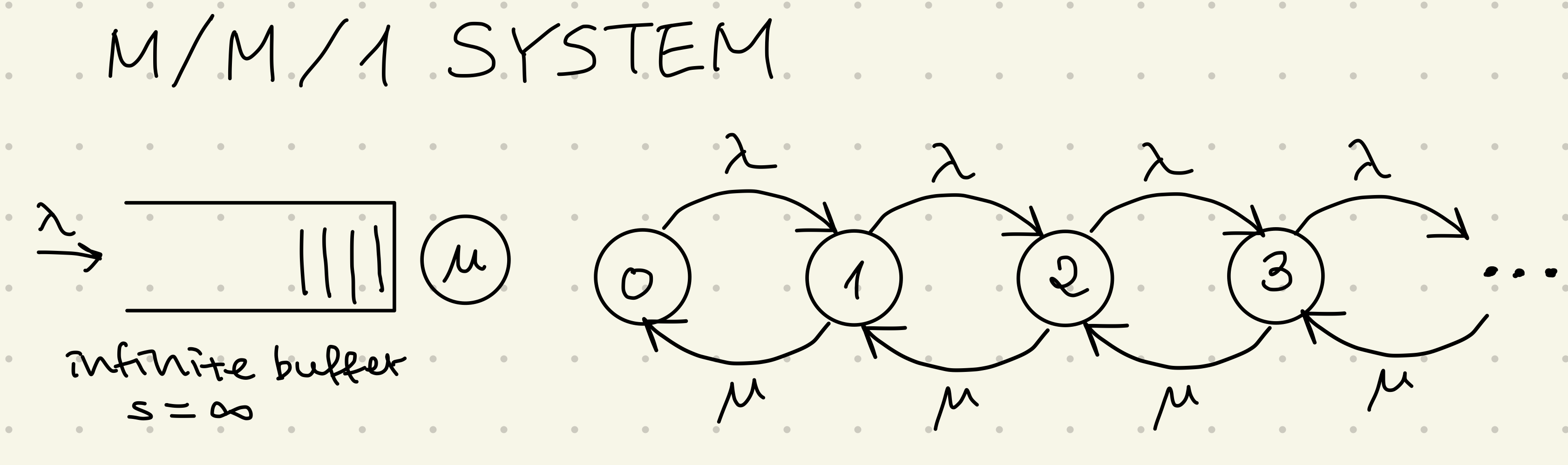
- Arriving requests are distributed according to a Poisson process with intensity \(\lambda\) and get a service of exponential duration with parameter \(\mu\)
- One server & an infinity queue ( \(s = \infty\), waiting system )
- Model for \(X(t)\) : birth-death-process iwth birth-rate \(\lambda\) and death-rate \(\mu\)
We can now draw the state transition diagram. It is shown on the upper right side. For the birth rate, \(\lambda\) is the same for all state transitions regardless if it is an occupation of the server unit or a buffer unit. For the death rate, we have to distinguish between state transitions between occupied server units and filled buffer units. For the server units the state transition probability rises with more server units being in use. For filled buffer units the state transition probability stays the same. In this case of one server units all death rates are the same and equal to the departure rate \(\mu\).
| utilization | state probabilites | mean number of occupied state |
mean delay of a packet |
| $$ \rho = \cfrac{\lambda}{\mu}$$ | $$ p(X=0) = (1 - \rho)$$ $$ p(X=1) = (1 - \rho) \rho$$ |
$$ L = E[X] = \sum_x x p(x) = \cfrac{\rho}{1 - \rho}$$ | $$T_D = \cfrac{L}{\lambda}$$ |
| mean queue length | mean waiting time | ||
| $$\Omega = E[X] - E[X_{server}] = \cfrac{\rho}{1 - \rho}$$ | $$T_W = \cfrac{\Omega}{\lambda}$$ |
Using Little's Law we can calculate the mean delay of a packet \(T_D\) and the mean waiting time \(T_W\). It is the respective mean value divided by \(\lambda\)
Next, we look at an M/M/N queueing system. The difference to the system before is that we have N server units now. This is illustrated in the left side figure.
M/M/N Queueing System (N servers)

In this case the departure related state transitions, the death rates, depend on the actual number of packets in the system.

From the left to the right the state transition probability increases by a factor of the departure rate that is the actual number of occupied server units. That means the probability of completing the processing of a packet increases with the number of used server units.
- The death rate depends on the actual number of packets in the system.
| $$ A = \cfrac{\lambda}{\mu} = \lambda h$$ | state probabilities | "Erlang Waiting Formula" $$ P_W = \cfrac{\cfrac{A^N}{N!} \cfrac{N}{N-A}}{\sum^{N-1}_{i=0} \cfrac{A^i}{i!} + \cfrac{A^N}{N!} \cfrac{N}{N-A}} $$ |
| $$A = N \rho$$ | $$ p(x) = p(0) \cfrac{A^x}{x!} $$ $$ for x= 0,1,...,N $$ |
|
| $$\rho = \cfrac{A}{N} $$ | $$ p(x) = p(0) \cfrac{A^N}{N!} \cfrac{A^{x-N}}{x!} $$ $$for x= N, N+1, ... $$ |
|
| $$A < N$$ | $$p(0) = \cfrac{1}{\sum^{N-1}_{i=0}{\cfrac{A^i}{i!}} + \cfrac{A^N}{N!} \cfrac{N}{N-A}} $$ | mean queue lengh $$\Omega = p(N) \cfrac{\rho}{1- \rho}$$ |
| mean waiting time $$ T_W = \cfrac{\Omega}{\lambda} $$ |
As a last example, M/M/N/0 loss system.
M/M/N/0 Loss System
as same as M/M/N System, we have N server units here but zero buffer. This means that packets do not wait in a buffer, but packets arriving when all server units are occupied get lost.

- N servers and no buffer units : Loss System
- no waiting, but loss
| "Erland Loss Formula" $$ B = p(N) = \cfrac{\cfrac{A^N}{N}}{ \sum^N_{k=0} \cfrac{A^k}{k!}} $$ |

'All About ECE > Communication Networks' 카테고리의 다른 글
| [Commu-Network/정보통신망] Message Transfer : Nachrichtenaustasuch (2/2) (0) | 2023.01.28 |
|---|---|
| [Data Networking] MAC and PHY layers (0) | 2023.01.16 |
| [Data Networking] Performance Analysis - a brief introduction (0) | 2023.01.14 |
| [Data Networking] Protocols, OSI Protocol Stack (0) | 2023.01.13 |
| [Commu-Network/정보통신망] Message Transfer : Nachrichtenaustasuch (1/2) (0) | 2022.12.25 |


댓글